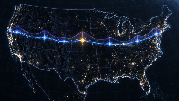
The Weather at the Hour You Get There

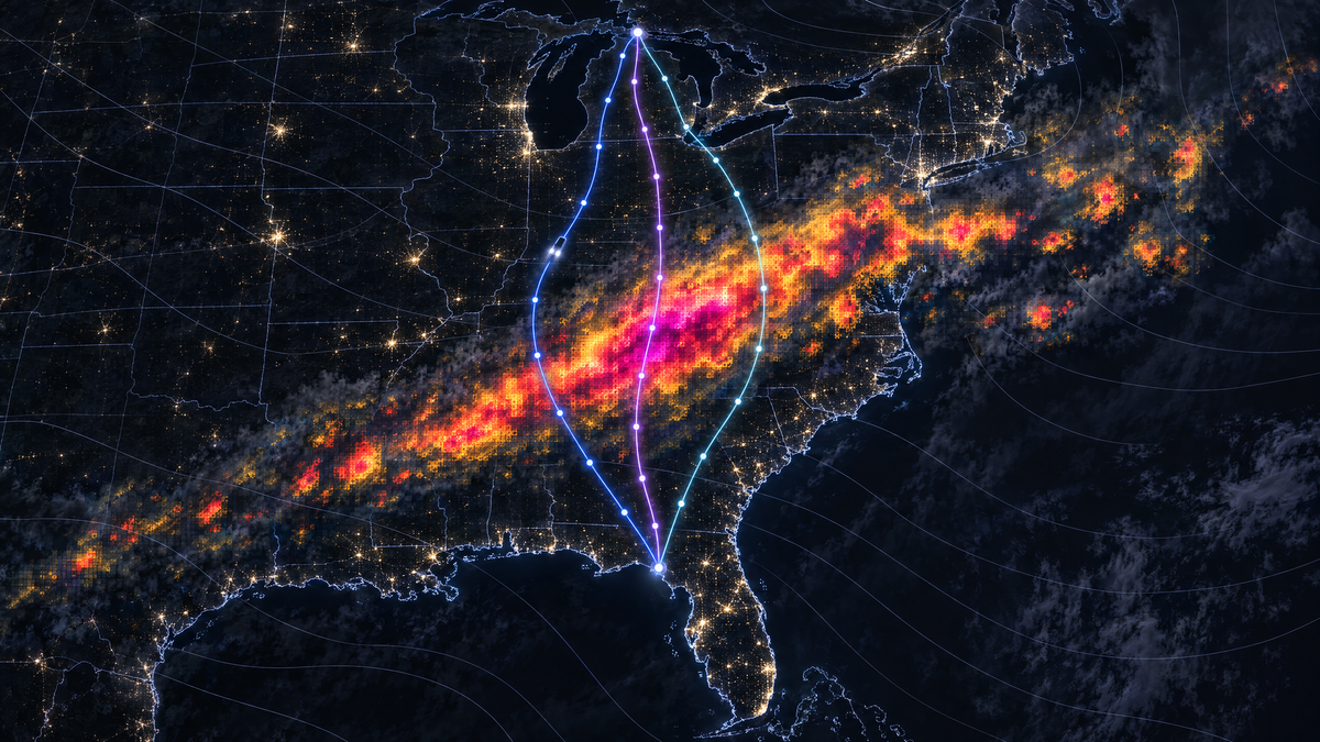
At seven in the evening on Tuesday, 3 November 2026, the forecast for downtown Chicago was calm: wind 10.6 mph, gusts to 22.8, no rain. A truck leaving for Atlanta at that hour with 42,000 pounds on board would pass any weather check made at the dock. On one of the three good routes south, the same truck reaches mile 420 at 01:33, on I-24 in western Kentucky. Rain is falling there at 0.38 inches an hour, and the next three checkpoints are High too.

None of that shows at the dock, because the dock is the wrong place and seven is the wrong time. The question a dispatcher has is narrower and harder: what weather will this truck drive through, on this road, at the hour it reaches each part of it? Squall Line is a web app that plans up to three truck routes, follows each one through time, reads the forecast at every checkpoint for the hour the truck gets there, turns wind, rain and snow into a risk level, recommends a route and says why, and paints the weather over the whole corridor as a heatmap you can play or drag through 48 hours. It runs at squall-line.vercel.app.

For that Chicago evening it compares routes of 703, 722 and 763 miles. The longest meets 60 miles of High rain, the middle one 10, the shortest none, and the card on top gives the reason in one line: "Next best is route B: 10 mi of High, against 0." The forecast is the one Open-Meteo gave at 12:12 that day. The app keeps the plan as a recording, so the storm can be replayed at /?demo=storm long after the rain has moved on. All times in this post are Chicago time.

The question, stated precisely

A route is a curve on the map. A trip is a curve through space and time. Write the truck's position as a function of time, x(t), from the departure t₀ to the arrival. The forecast is a field over space and time, F(x, t): wind, rain and snow at every place and hour. What the truck meets is F along its own path, F(x(t), t).

Two shortcuts miss it, in different ways. The forecast at the dock, F(x(t₀), t₀), is the first point of that curve and says little about the rest. A map of the forecast at the departure time, F(x, t₀), has every place on the route and the wrong hour for all of them but the first: it shows where the rain is at 19:00, not where it is when the truck gets there.

Measured along the road, with s the mile and t(s) the moment the truck reaches it, the risk at mile s is r(s), the level of F(x(s), t(s)) for the truck's load. What a dispatcher can compare is the miles a route spends at each risk level ℓ:

miles(ℓ) = ∫ [ r(s) = ℓ ] ds

The integral runs over the route, from mile 0 to its length D, and the bracket is 1 where the condition holds and 0 elsewhere, so the five numbers add up to D. Each part of the planner supplies one term of that integral:

• x comes from a truck routing engine, because a truck's road is not a car's.
• t comes from the engine's own timing plus the federal hours-of-service rules, because a driver has to stop, and every hour after a stop moves.
• F comes from an hourly forecast, read the way each field is defined, at the place and the hour.
• level comes from the app's rule table, which turns wind, rain, snow and the load into one of five levels.
• The integral is computed at checkpoints, each standing for a stretch of road, and routes are compared on the result in a strict order that names its reason.

The heatmap is the same field drawn over the whole corridor, so you can see what the checkpoints sampled and what is moving next to them.

Routes that actually differ

The primary engine is TomTom's truck routing. It is asked for the fastest route and two alternatives for the truck as it is: travelMode=truck with the gross weight, the governed speed, the length, width and height, and the departure time with traffic. The truck is a tractor with a 53-foot trailer, 21.9 m long, 2.6 m wide and 4.11 m high, with a tare of 35,000 lb for the tractor and an empty dry van, so the recorded trip runs at 77,000 lb gross, just under the 80,000 lb federal limit on the Interstate System. Its governor is set to 65 mph, the most common factory setting (24.8% of 332,530 vehicles) in the data behind the 2016 federal speed-limiter proposal.

Without a TomTom key the planner still routes trucks. Valhalla has a truck costing that takes the same weight, size and top speed; its public server refuses trips longer than 1,500 km in a straight line, so the planner sends it only trips of up to 900 miles as the crow flies. Past that, or when Valhalla does not answer, OSRM's public server answers with car routes, and no segment is driven faster than the truck's 65 mph. The planner turns all three answers into the same shape, so the rest of the pipeline treats them alike. The recorded storm was routed by Valhalla, which returned all three routes in one call.

An engine's alternatives can be the same road with a different exit. To tell real alternatives from near-copies, each route is sampled every tenth of a mile and reduced to the set of grid cells it passes through, cells of 0.004° (about 400 m). The overlap of route a with route b is the share of a's cells that lie within one cell of b. It is not symmetric, and the planner always measures it from the candidate's side: how much of the new route's own road is already taken.

• An engine's alternative is dropped only when 97% or more of its road is already on a faster route.
• When fewer than three routes remain, the planner routes through a point to one side of the fastest route's midpoint, then the other side, offset by a seventh of the trip's straight-line length (kept between 15 and 120 miles). Such a route is kept only if less than 80% of its road is shared with each route already chosen and it takes at most 1.5 times as long as the fastest.
• Places with only one or two reasonable roads between them get one or two routes, and the page says so.

The two thresholds differ on purpose. An engine's alternative is a route the engine already rates, so only a near-copy goes. A route forced through a side point has to be clearly different, and not absurdly slow.

Routes are named by their two main roads, the ones with the most miles: route C here is "I-24 · I-57". When two routes share both, each gets the road that tells it apart, the one it drives at least 5 miles more on than its twin. A live plan from Kansas City to Minneapolis comes back as "I-35 · US-69 via I-235" and "I-35 · US-69 via US-65".

Checkpoints, and the miles they stand for

A checkpoint goes every 10, 25 or 50 miles from the origin, and the destination is always one. A regular mark closer to the destination than a tenth of the interval is dropped, so the last stretch is never a sliver. Positions are found by distance along the route's polyline, rescaled to the engine's own route length, so mile 420 on the map is mile 420 on the engine's odometer.

Each checkpoint stands for the road halfway to each neighbour; put another way, every mile takes the level of its nearest checkpoint. At a 10-mile interval the first checkpoint stands for 5 miles and most of the others for 10, and the represented miles of all checkpoints add up to the route's length exactly. A property test checks that for any length from half a mile to 3,000 miles at every interval. Those are the weights of the trapezoidal rule, so the miles at each level are a quadrature of the integral above.

For the recorded trip, route A has 72 checkpoints. Its miles add up to 682.9 Low and 20 Moderate, 702.9 in all.

When the truck gets there

Arrival times start from the engine's own clock. Every engine reports driving times along its route: TomTom per instruction, Valhalla per maneuver, OSRM per segment of the polyline. Between two of those points, time is spread over the polyline in proportion to distance. That keeps the engine's knowledge of slow city miles and fast interstate miles, which a single average speed would erase.

Then the law adds its stops. For a property-carrying driver, 49 CFR 395.3 says that "A driver may not drive without first taking 10 consecutive hours off duty", that "A driver may drive a total of 11 hours", and that "driving is not permitted if more than 8 hours of driving time have passed without at least a consecutive 30-minute interruption in driving status." The planner applies the two that bind on a long trip: a 30-minute break once 8 hours of driving have passed without one, and a 10-hour rest after 11 hours of driving, which starts the next shift and also counts as the break. With no other on-duty time a shift is 8 h + 30 min + 3 h = 11.5 h, inside the 14-hour window, so the window never binds. The driver is assumed to start rested, with hours left in the week.

Route A of the recorded trip shows what that does. The engine says 11 h 52 m of driving:

Tue 19:00  drive 8 h
Wed 03:00  break, mile 475.6
Wed 03:30  drive 3 h
Wed 06:30  rest, mile 657.7
Wed 16:30  drive 52 min
Wed 17:22  Atlanta

The break comes at the eight-hour mark, the rest at the eleven-hour limit, in north Georgia, and the trip takes 22 h 22 m. Every checkpoint after the rest is reached ten and a half hours later than the engine's clock alone would say, and its forecast is read for that hour. A planner that skips the rest reads the last 45 miles at dawn and the truck drives them in the afternoon.

The rules also have an exception that a weather planner should leave alone. 49 CFR 395.1(b) allows up to two extra hours of driving in adverse driving conditions, and 395.2 defines them as conditions "that were not known, or could not reasonably be known" to the driver before the duty day or to the carrier at dispatch. A planner that reads the forecast before dispatch makes the weather known, so it does not budget those two hours.

Reading the forecast as it is written

The forecast comes from Open-Meteo's hourly API with the best_match model. Over the contiguous US that is NOAA's HRRR, a 3-km model that runs every hour and out to 48 hours four times a day, and then NCEP's GFS, a global model at about 13 km. One request asks for every location of the plan at once: wind speed and gusts at 10 m, rain, showers, snowfall, temperature and the weather code, in mph and inches.

Open-Meteo's hourly fields come in two kinds, and its documentation says which is which. Wind speed and temperature are "Instant", a value at the stamped time. Rain, showers and snowfall are a "Preceding hour sum", and gusts a "Preceding hour max": the value stamped 02:00 describes the hour from 01:00 to 02:00. So at an arrival time t the planner reads them differently:

• instant fields are interpolated linearly between the hours on either side of t, and the weather code, a category, comes from the nearest hour;
• preceding-hour fields are read from the hour that contains t, the one stamped at the first full hour after it.

Here is the recorded series at route C's mile 420, where the truck arrives at 01:33:

The first reading is the rain that fell there between midnight and one, while the truck was still 36 to 100 miles back, crossing from Illinois into Kentucky. The second averages that past hour into the present. Only the third is the rain the truck drives into. Wind, being instant, is interpolated: 9.5 mph at 01:00 and 9.7 at 02:00 give 9.6 at 01:33.

Three more details:

• Rain is rain + showers. Open-Meteo's showers is convective precipitation, reported apart from rain by models that separate the two, such as GFS; reading rain alone would miss thunderstorms there.
• Snowfall is fresh snow depth. With precipitation_unit=inch it is inches of snow per hour, which is the unit of the rule table.
• Values are classified at the precision they are shown in, 0.1 mph and 0.001 in/hr, with one rounding rule on the server and in the browser. In binary floating point, 0.09 + 0.01 is 0.09999999999999999, which a bare < 0.10 calls Low while the page shows 0.100. Rounding first makes the level match the number on the screen. A missing value is an error, never Low.

From weather to risk

The rule table is the app's configuration. The server publishes it at /api/rules, and the browser draws its legend, its rules panel and its own classifier from that answer, so there is one table.

Every band includes its lower bound, so 25 mph is Moderate and 0.25 in/hr is High. Rain and snow are the exception at the top: No Travel starts above 1.00 in/hr and above 3.0 in/hr, so 1.00 in/hr is still Severe while 55 mph of wind is already No Travel. The worst of wind, rain and snow sets the checkpoint's level.

Heavy loads raise the wind level. With more than 40,000 lb on board, 35 to 44 mph is Severe instead of High; with more than 30,000 lb, 45 to 54 mph is No Travel instead of Severe. Wind at 55 mph and over is No Travel for any load. In the storm these rules never fire: the strongest wind anywhere in the corridor over the 48 hours is 29.9 mph.

The table's lines are not the weather service's. The Federal Meteorological Handbook calls rain light "Up to 0.10 inch per hour", moderate "0.11 inch to 0.30 inch per hour" and heavy "More than 0.30 inch per hour", so 0.10 in/hr is light rain to the handbook and Moderate to the table, whose High starts at 0.25, below the handbook's heavy. The National Weather Service's typical criteria for a Wind Advisory are "Sustained wind speeds of 30 to 39 mph lasting for 1 hour or longer", and for a High Wind Warning "sustained wind speeds of 40 mph or greater lasting for 1 hour or longer, or winds of 58 mph or greater for any duration"; the table's High starts at 35 mph, inside the advisory band.

A ranking that says why

Each route's exposure is the miles it spends at each level, plus the mile-weighted average level, from 0 for Low to 4 for No Travel. Routes are ranked by five keys, in order: the fewest No Travel miles, then the fewest Severe miles, the fewest High miles, the lowest average risk and the shortest trip time.

This is a lexicographic order: the first key on which two routes differ decides. A weighted sum would set an exchange rate between hazard and time, so many minutes saved for one mile of High. This order refuses to set one: no amount of time saved buys back a mile at a worse level. No Travel miles come first because a route through No Travel weather cannot be preferred to one without it, however the other keys compare. When every route meets No Travel weather, the plan still ranks them and says that no route is safe.

A strict order has a practical virtue: the reason for every ranking is one comparison, and the card names it. Miles are compared to a tenth of a mile, the average to a hundredth and the trip time to the minute, the precision each is shown at, so the reason can always be read off the numbers on the screen. For the recorded storm:

The first two keys tie, and High miles decide. On a calm day every route is Low all the way, the first four keys tie, and the fastest route wins. That is what a live plan from Kansas City to Minneapolis did early on the afternoon of 3 November, with 30,000 lb: every checkpoint Low, routes of 444, 458 and 550 miles, and the 444-mile route on top.

The storm does not show the order at its hardest, because there the safest route is also the shortest and the fastest. The same Kansas City trip did, two hours later. Planned at 16:06 for a 17:00 departure, with a checkpoint every 25 miles, it came back with the 444-mile route on I-35 and US-69 last: 25 miles of High rain in central Iowa at 21:18. The 554-mile route on I-29 and US-75, Low all the way, came first, although its trip takes 9 h 36 m against 7 h 21 m. A weighted sum would have had to decide whether 2 h 15 m is worth 25 miles of High.

The hazard list merges consecutive checkpoints at High or worse into stretches with their miles, the arrival time at the stretch's first checkpoint and the cause. Route C has three, all rain: miles 415 to 455 from 01:33, 475 to 485 from 02:29, and 585 to 595 from 04:43.

The corridor heatmap

The checkpoints say what each truck meets. The heatmap shows what is around it: the weather over everything within a distance W of any route, where W is 4% of the longest route, kept between 30 and 90 km. For the recorded storm W is 49.1 km. The ranking never reads the map; the map is there to watch the weather move.

One grid, in the map's projection. The corridor is covered by a regular grid in Web Mercator, the projection the map is drawn in. Each cell inside the corridor is one forecast location, and the cell size is chosen so that those cells nearly fill a budget of 120 to 200 locations, whatever the checkpoints leave of the plan's 450. The recorded storm has 198 cells inside a lattice of 17 × 33. The plan carries 49 hourly frames of wind, rain, snow and risk for every cell, from hour 0 to hour 48. Because the grid is regular in the map's own projection, the whole lattice is one image, a canvas pinned to the map by its four corners, and every cell lands where its forecast was taken. A grid regular in latitude would not: drawn the same way over this corridor, from 33.2° N to 42.3° N, its rows would land up to 16 km from where they belong, half a row.

Fifteen pixels a cell. Each cell is drawn as 15 × 15 pixels, so the image is 255 × 495. Every pixel takes its weather from up to four cell centres with bilinear weights that sum to one, and from the two hourly frames around the clock, linearly in time. Only then is the blended weather classified, with the server's own rules and the truck's load. The pixel weights are computed once per plan; a frame only blends and classifies.

Blend, then classify. The order matters because classification is a step function, and a step function does not commute with averaging. Take a block of four neighbouring cells on the Kentucky–Tennessee line north of Nashville at 08:00 on Wednesday, hour 13 of the trip. Their rain is 0.000, 0.043, 0.028 and 1.331 in/hr: three Low cells and one No Travel cell. Blending colours or levels between them invents a gradient that has nothing to do with rain. Blending the rain does not. Along the diagonal from the dry corner to the wet one, the blended rain crosses 0.10 a quarter of the way along, 0.25 at 42%, 0.50 at 60% and 1.00 at 86%, so the pixels pass through Moderate, High, Severe and No Travel in order, each where the estimated rain crosses its threshold. At the middle of the block every weight is a quarter: the blended rain is 0.35 in/hr, High, where averaging the four levels would give Moderate. As the clock moves, the same blend runs between hourly frames, so the bands grow, shrink and drift instead of jumping from hour to hour.

Exact where the forecast is. Fifteen is odd on purpose: one pixel's centre sits exactly on each cell's centre. There the bilinear weights are one and zero, and on the hour the time weight is too, so that pixel shows the cell's own forecast and the level the server computed. Unit tests check it at every cell on every hour of two recorded plans, 9,702 cell-hours for Chicago to Atlanta alone, both in the classifier and in the painted pixel itself, and another test makes sure that plan covers every level, so the check means something. With an even number, no pixel would sit on a centre, and a single cell just over a threshold, with drier neighbours, could vanish from the map.

An edge that follows the roads. The image's edge follows the band within W of the routes, not the cells' staircase. Each pixel's distance to the nearest route is found by walking the routes in steps of a pixel or two and stamping each step as a capsule, instead of measuring every pixel against every route point. The edge fades over 22% of the half-width, inside and out.

Fast enough to drag. Low is clear, so the corridor only lights up where the rules do. Computing the pixels of one frame of the risk layer takes a median of 2.4 ms (p95 2.5 ms) for the stormy corridor, measured over 960 frames in headless Chromium; a 60 Hz screen allows 16.7 ms a frame, and the canvas upload and the map's redraw come on top. CI keeps the median under 12 ms. Play runs the clock at four hours a second, so two days pass in twelve seconds; the trucks move along their routes with it. The wind, rain and snow layers use colour ramps keyed to the same thresholds.

A free forecast with a quota per address

Open-Meteo's free API allows "Less than 10'000 API calls per day, 5'000 per hour and 600 per minute", counted per IP address, and every location in a request counts as a call. A plan asks for at most 450 locations: the corridor's cells plus the checkpoints of all three routes. When the checkpoints would not fit, they are snapped to a coarser grid, first those more than 48 hours ahead (to 0.125°, about the 13 km of the GFS that forecasts them anyway), then the nearer ones, step by step. Each location's series is cached for half an hour, so the same trip with another load costs no new forecast request; another interval moves the checkpoints and the grid, and another departure needs hours the cache seldom holds. Even so, at 450 locations one address affords one fresh plan a minute, 11 an hour and 22 a day, and a cloud function shares its address with whatever else runs there.

So the server keeps the quota headers of every answer, and it does not send a request the remaining quota cannot cover: Open-Meteo would admit it and then hold it until the quota refills. Instead, and whenever Open-Meteo refuses or does not answer in time, /api/plan answers 503 with the exact Open-Meteo query. The browser sends that query from its own address, where the quota is its own, and asks for the plan again with the answer attached. The query lists every location the plan needs, even those this server process has cached, because the second attempt can reach another process with a cold cache. The server still computes the plan. It validates the supplied answer and uses it for that one request: it never enters the shared cache, so no browser can put weather into anyone else's plan. The price is that, for that one plan, Open-Meteo sees the user's address instead of the server's.

Tests that never touch the network

The backend has 258 tests covering 98% of its statements and branches, with mypy in strict mode and ruff. The core of them is three recorded trips: Chicago to Atlanta (routed by Valhalla), Denver to Salt Lake City (recorded with OSRM) and Sacramento to Reno (Valhalla), each with the Open-Meteo answer it got. A replay transport answers each request with the next recorded exchange, after checking that it is the request that was recorded. The whole pipeline runs offline and gives the same answer every time, and a change in what the planner asks for fails the test instead of silently answering a different question.

Property tests cover the invariants: polylines survive encoding and decoding, and the vectorized classifier the heatmap uses agrees with the scalar one the checkpoints use for any wind, rain, snow and load.

The browser has 94 unit and component tests, among them the cell-by-cell check against the server. The frontend's recorded plans are the backend's own output for the same recordings, and a backend test fails if they drift. Playwright runs the production build against a mocked API and mocked map tiles on a desktop viewport (1440 × 900) and a Pixel 7: 29 runs. GitHub Actions runs all of it on every push to main and every pull request, with backend coverage held at 95% or more.

The backend is Django 6.1 with django-ninja and NumPy on Python 3.14; the browser is React 19, TypeScript 7, Vite 8, MapLibre GL 6 and Tailwind 4. It is deployed on Vercel: the Vite build as static files and the Django API as one Python function.

What it doesn't do

• The whole week of a driver. There is no sleeper-berth split and no 60- or 70-hour weekly limit, and no on-duty time besides driving.
• Probabilities. It reads one deterministic forecast, the best match for each place. A forecast for tomorrow night is less certain than one for tonight, and the app does not say by how much. The heatmap's hours count from the departure, so for a trip planned ahead its last hours can fall beyond the HRRR's 48 and come from the coarser GFS.
• Everything that makes a road dangerous. Gusts are shown but not scored, and there is no visibility, fog, freezing rain, ice on the pavement or lightning. Snow is depth per hour, not road condition.
• Weather that slows the truck. Times come from the engine and the hours of service, so rain never slows the modelled truck, and a truck slowed by rain would reach the later checkpoints later than planned. A plan is made at dispatch, with no re-planning on the road; traffic is what the engine expects for the departure time.
• Routing around the weather. The routes come from the engine and the side points. The planner compares good routes; it does not search the road network for the driest one.
• Fine sampling. At 65 mph, ten miles take about nine minutes, finer than the forecast's hours, but ten miles is coarser than a 3-km model, and a storm cell narrower than the spacing can sit between two checkpoints. Between hours the map blends precipitation linearly, while a checkpoint reads the hour that contains its arrival.

What generalizes

Take the trucks away and the shape remains: something moving along a path, through a field that changes in time, judged by thresholds.

• Sample the trajectory, not the place. The forecast at the start is one point of the curve. Put time on the path first, then read the field.
• Read data as it is defined. An instant value, a preceding-hour sum and a preceding-hour maximum are three different things at the same time stamp.
• Classify last. Interpolate the measured quantity, then apply the thresholds. Interpolated colours and levels describe no weather at all.
• Keep one table. Publish the rules once, let the server and the renderer read the same copy, and test that they agree at every sample.
• Make the reason a key. A lexicographic order gives up trade-offs and gets a one-line explanation the user can check on the screen.
• Put the quota where the user is. When a free API counts per address, let each user's browser carry its own share, and never let what one supplies reach anyone else.
• Record, replay and check the question. A replay that verifies each request tests the questions the code asks, not only the answers it gets.

The code and the tests are on GitHub; the app is at squall-line.vercel.app.

References

• Electronic Code of Federal Regulations, 49 CFR 395.3, Maximum driving time for property-carrying vehicles; 49 CFR 395.1 and 395.2 on adverse driving conditions.
• 23 CFR 658.17, Weight: the 80,000 lb gross limit on the Interstate System.
• NHTSA and FMCSA, speed limiting devices, notice of proposed rulemaking, 81 FR 61942, 7 September 2016.
• Open-Meteo, Weather Forecast API documentation (variables and their valid times, best_match) and terms (the free tier's limits).
• NOAA Global Systems Laboratory, The High-Resolution Rapid Refresh (HRRR).
• NOAA NCEP Environmental Modeling Center, Global Forecast System (GFS).
• OFCM/ICAMS, Federal Meteorological Handbook No. 1, Surface Weather Observations and Reports, FCM-H1-2019, table 8-1.
• National Weather Service, Instruction 10-515, WFO Non-Precipitation Weather Products Specification, 16 May 2025.
• TomTom Routing API, Calculate Route; Valhalla route API; OSRM; MapLibre GL JS.