The Cheapest Way Across America

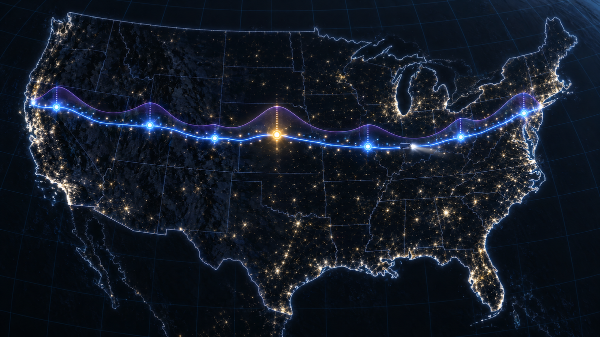
On Interstate 80 near Overton, Nebraska, there is a truck stop listed at $2.899 a gallon, as cheap as it gets within five miles of the road between New York and Los Angeles. A truck crossing the country on a 500-mile tank should roll in there on fumes and leave with all 50 gallons. On the way, it should arrive empty at three stops in a row, Overton the last of them, because each is cheaper than the one before. And at its last stop, on I-15 in the Nevada desert, it should buy exactly 18.49 gallons: with what is left in the tank, that covers the 314.2 miles to Los Angeles and not a mile more.

None of that is a rule of thumb: most of it falls out of a small piece of mathematics with a name, the gas station problem. This post is about that mathematics, the two places where real roads break it, and the systems work around it: fuel-route-api, a Django API that takes any start and finish in the USA and returns the route, the stops and the fuel bill after one call to a routing engine.

For New York to Los Angeles it answers: 2,810 miles of road, 362 truck stops within five miles of it, seven fuel stops, $711.08 of fuel bought on the way. Finding the stations and choosing the stops takes about 15 milliseconds. The strictly cheapest plan is one parameter away: 13 stops to save $3.71.

The problem, stated precisely

Put the route on a line from mile 0 to mile L. Station i sits at mile xᵢ, a detour dᵢ off the road, and sells fuel at pᵢ dollars a gallon. The tank holds C gallons, here 50 (500 miles at 10 miles per gallon), and every mile burns a tenth of a gallon. The vehicle starts with F₀ gallons, a full tank by default, may buy any amount at a stop and must never run dry. Minimize the fuel bill. The vehicle's numbers are query parameters of the API: max_range_miles and mpg set the tank, start_fuel_gallons sets F₀, and end_fuel_gallons asks for fuel left at the finish.

Without detours this is a linear program over the amounts bought, gᵢ gallons at station i. The fuel on arrival, fᵢ, is linear in them. Count the finish as one more station with nothing for sale; then every arrival must be at least empty and every departure at most full:

minimize   Σ p_i·g_i
over       g_i ≥ 0
where      f_i = F0 − x_i/mpg
               + Σ_{j<i} g_j
subject to f_i ≥ 0
           f_i + g_i ≤ C

Operations research calls it the fixed-route vehicle refueling problem; Lin, Gertsch and Russell treat it as a special case of the inventory-capacitated lot-sizing problem (ordering stock over time into a warehouse with a limit) and give a linear-time algorithm. In algorithms it is the gas station problem, after Khuller, Malekian and Mestre's paper "To Fill or Not to Fill": their algorithm for a fixed path is greedy and runs in O(n log n) time, and the paper goes on to general road graphs with a limit on the number of stops, a case Papadopoulos and Christofides later sped up.

The greedy fits in a few lines:

at each station:
  if a cheaper station or
  the finish is in range,
    buy just enough to reach
    the first of them;
  otherwise fill up.

Why the greedy is right

Here is a short way to see it; it is a sketch, not the papers' proofs. Fuel has no identity, so account for it first in, first out, with the starting fuel burned first and free. A gallon is then burned before anything bought after it, and the tank never holds more than 500 miles of fuel, so every gallon is gone within 500 miles of its pump. Every mile driven on bought fuel is therefore paid for at no less than the lowest price among the stations in the 500 miles behind it. That is a lower bound no plan can beat.

The greedy meets the bound. It never carries fuel past a cheaper station it could reach, and it fills up only where nothing within a full tank ahead is cheaper, so every mile burns fuel from the cheapest station in its window. Past the miles the starting fuel covers, the optimal bill is the integral along the route of a sliding-window minimum of the price:

cost = (1/mpg) · ∫ w(m) dm,
       m from s to L
w(m) = min { p_i :
         m − R ≤ x_i ≤ m }

Here R is the range, 500 miles; s is the distance the starting fuel covers; and w(m) is the lowest price among the stations in the R miles behind mile m.

This is the plan the API returns for New York to Los Angeles. The stops come from the dynamic program described below; what each one buys follows the greedy rule to the gallon:

The trip burns 281.05 gallons; 50 were in the tank at the start, so the plan buys 231.05 gallons for $711.08, an average of $3.08 a gallon. The 362 stations along the way range from $2.899 to $4.132, with a median of $3.462: the same gallons at the median price would cost about $800.

Thirteen stops to save $3.71

The argument above has two quiet assumptions. Both fail on a real interstate.

Stops are free. The window-minimum plan stops wherever the minimum changes, and when prices drift slowly along the way, down or up, it changes often. Khuller and colleagues note that with prices decreasing toward the destination, the cheapest solution "may involve an arbitrarily large number of stops". Coast to coast, the strictly cheapest plan makes 13 stops and costs $707.37. Two of those stops buy less than five gallons, and one of them comes 18.6 miles after the stop before it. Six extra exits, ramps and pumps. Suzuki's 2008 model of motor-carrier fuel purchasing makes the same complaint about commercial fuel optimizers: they "minimize only the fuel cost, and ignore or underestimate other costs".

Stations are on the road. A truck stop three miles off the interstate costs six miles of fuel to use, 0.6 gallons, however much is bought there. That makes its effective price fall as the purchase grows, so posted prices no longer rank stations: a cheap pump down a side road can lose to a dearer one at the exit for a small purchase and win for a large one.

Both are fixed charges, the setup costs of lot sizing, and an argument that prices miles one at a time has no place for either. The planner prices both. The detour is fuel, so it is charged as fuel. The stop itself costs something besides fuel, so the planner charges each stop a stop_penalty, $5 by default, when it chooses stops. The reported cost is fuel only, and stop_penalty=0 gives the strictly cheapest plan.

Whether a stop is worth it now depends on how much you will buy there, which depends on how much fuel you arrive with. The greedy ranks stations by price alone, so the fuel level has to become part of the state.

A dynamic program over fuel

The planner measures fuel in steps of a quarter mile of range (0.025 gallons at 10 miles per gallon), so a 500-mile tank is K = 2,000 steps, with levels 0 to K. It walks the stations in route order and keeps one array:

cost[f]: least cost
  to be here with f steps
  (0 at the start level,
  ∞ at every other level)

drive δ steps:
  cost[f] ← cost[f + δ]
  (∞ when f + δ > K)

stop at station i:
  c, b: detour in, out
  u: price of one step
  arrive with a = f − c
  leave with t > a:
  leave[t] = min over a < t
    of cost[a + c]
       + (t − a)·u
       + penalty
  rejoin with t − b

merge:
  cost[f] ← min(cost[f],
                leave[f + b])

The detour in is driven before buying and the detour out after, so the tank's limit applies at the pump.

Written that way, each station looks quadratic in K: every leaving level against every arrival level. It is not, because the price is linear in the amount bought. Split the cost of a purchase into a part that depends only on the arrival level and a part that depends only on the departure level:

cost[a + c] + (t − a)·u
  = (cost[a + c] − a·u)
    + t·u

g[a]     = cost[a + c] − a·u
leave[t] = t·u + penalty
           + min g[a],
             a ≤ t − 1

The remaining minimum is a prefix minimum of a single array: one numpy.minimum.accumulate, plus a second scan that records which arrival level attains each prefix minimum. In min-plus terms, buying fuel is a convolution of the cost array with the kernel k·u for k steps bought, and a linear kernel collapses the convolution to a scan. A station costs O(K) vector work and the whole route O(n·K). For New York to Los Angeles that is 362 stations times 2,001 levels, about 724,000 cells, and NumPy finishes in about 10 milliseconds.

One number per level is enough because fuel is fungible: the cost of the rest of the trip depends on where the vehicle is and how much it holds, not on what it paid for it. That is the principle of optimality at work.

Each station stores two arrays, whether it stopped at each level and the arrival level it came from, and the stops come from walking those decisions back from the finish. The walk must land exactly on the starting fuel level; if it doesn't, the code raises instead of returning a plan.

Khuller and colleagues point out that discretizing fuel "only yields a pseudo-polynomial time algorithm". Here the resolution is a constant, not a function of the input: a quarter mile of range is finer than the data deserves (nearly half the stations are only known to the town), and K depends only on the range: 2,000 steps whatever the route. With no detours, no penalty and every distance on the grid, the dynamic program reproduces the greedy's optimum; with detours and a penalty, it is still exact on its grid. A mixed-integer solver would also find the optimum, and the tests below use one, but how long branch and bound takes depends on the instance; the dynamic program always costs n·K.

Making the grid honest

The planner gives the grid one task, choosing the stops, and rounds in the safe direction.

Station positions are rounded to the nearest step, and the rounding error goes into the detours, which round up; the tank and the starting fuel round down. For a leg between two stops, the grid charges the road between their rounded positions, plus each detour padded by its stop's rounding: the way out of the first by however far that stop was rounded forward, the way into the second by however far that stop was rounded back. The padded leg therefore starts no later and ends no earlier than the exact one. No leg is shorter on the grid than on the road, and a plan that works on the grid works with the exact distances. On grid-aligned input nothing is rounded and the grid is exact. The price of this safety is small and explicit: a leg that would leave less than a mile of fuel to spare can count as out of range.

The amounts are not taken from the grid. Once the stops are chosen, the greedy rule computes them exactly, because for a fixed set of stops the greedy is optimal. A stop that ends up buying nothing is dropped, which removes its detour, and the amounts are worked out again. Put together, the guarantee is precise:

• the stops are optimal, for fuel plus penalties, on a copy of the instance that is slightly pessimistic, minus any stop that exact arithmetic shows to be unnecessary;
• the amounts are exact for those stops;
• the plan is feasible at the exact distances: replayed with them, it never arrives with less than nothing and never fills past the tank.

One more modeling trick: arriving with at least E gallons is the same problem as driving E × mpg miles past the finish, on a stretch with no stations. With the same fuel at the start and the finish, the bill covers every gallon the trip burns: Chicago to Denver with 25 gallons in and 25 out buys all 100.29 gallons in three stops, for $295.19.

When no plan exists, the API says why instead of guessing. If the starting fuel reaches neither a station nor the finish, it answers 422 start_fuel_too_low, with reach_miles and first_station_mile. If a stretch of road has no station within range, it answers 422 no_fuel_stop_in_range, with gap_start_mile and gap_end_mile.

Trusting the optimizer

The evidence for the recurrence is an independent solver that agrees with it on random instances. The test suite builds two.

• Without detours or penalty, the planner must equal the optimum of the linear program above, solved by scipy.optimize.linprog. Across 150 random instances, it does wherever the linear program has a solution and refuses wherever it has none.
• With detours and penalties, the problem becomes a mixed-integer program. Each station gets a binary stop flag yᵢ; gallons are allowed only where it is set (gᵢ ≤ C·yᵢ); the detour's fuel is charged only when stopping, with only the way in counted when the tank is checked at the pump; and the objective adds the penalty per flag. The planner must equal the optimum from scipy.optimize.milp. It does wherever a plan exists, across 140 random instances (60 of them with fuel required at the finish): routes of 300 to 2,500 miles, 3 to 17 stations, detours of 0, 0.5, 1 or 2.5 miles, prices from $2.80 to $4.20, starting fuel of 50, 30 or 12.5 gallons. Where no plan exists, both must agree on that too.
• With distances off the grid, across 150 more instances, every plan the planner returns is within 10 cents of the mixed-integer optimum, and replaying it with the exact distances never runs dry and never overfills. Where the planner refuses an instance, the test takes a mile off the range and a mile off the starting fuel and checks that the exact solver then finds no plan either.

Both oracles run on HiGHS, the open-source optimization software behind SciPy's linprog and milp. They share the model with the planner, not its algorithm.

pytest          # 109 tests
pytest -m live  # 1 real trip

The default run takes about 3 seconds with no network: HTTP is mocked, and one test replays a recorded route. The live run sends one real coast-to-coast request. Coverage is about 96%, and CI runs the suite on every push, on Python 3.12, 3.13 and 3.14 with Django 6.1.2 and Django REST Framework 3.18.3.

Finding 6,600 truck stops without coordinates

The price list has 8,151 rows of truck stop prices and not one coordinate. Its addresses describe highways, not streets: I-44, EXIT 283 & US-69. A street geocoder cannot resolve that, and geocoding thousands of addresses on every start-up would be slow and abuse free services.

The importer keeps every price row and gives each stop the mean of its prices. It also repairs mis-encoded names, the classic UTF-8-read-as-Windows-1252 damage that turns Stuckey’s into Stuckey’s.

Exit coordinates come from OpenStreetMap. Mappers tag highway exits as highway=motorway_junction nodes, with the exit number in ref, "as indicated on nearby signage". One Overpass query fetches every numbered junction in the contiguous US. Exit numbers restart in every state, so the number alone is ambiguous; the stop's town, from the Census, picks the junction with that number within 25 miles. For 375 stops another junction with the same number is also near the town, usually on another highway, and the nearest one wins. That puts 3,464 stops at their exit. The other 3,162 get their town's internal point from the Census Gazetteer (usually the centroid, moved inside the boundary when the centroid falls outside it), or from Nominatim for the 144 places the Census does not list. Those positions are approximate, and the API says so: every stop carries a location_precision of exit or town.

All of this runs once, ahead of time, in manage.py locate_stations: one Overpass query and about 150 Nominatim lookups. The result is committed to the repository as a CSV, and the importer reads it with the prices in about two seconds. A deterministic file is easier to review, test and diff than thousands of geocoding calls.

Stations along the route

OSRM returns New York to Los Angeles as 35,227 points. The planner needs, for every station near that line, two numbers: how far it is from the road and at which mile it meets it.

Latitude and longitude are a poor space for that question: a degree of longitude spans about 69 miles at the equator and about 52 at the latitude of New York. So the route and the stations become 3D points on a sphere of Earth's radius, in miles. There the straight-line chord between two points grows strictly with the great-circle distance between them, so the nearest point by chord is the nearest point on the sphere, and a five-mile radius becomes an exact chord limit. The route is resampled so no segment is longer than half a mile, and a KD-tree (Bentley's 1975 structure, here SciPy's cKDTree) is built over its points.

A bounding-box filter keeps the stations inside the route's bounding box, padded by the corridor width, and one batched query returns, for each, the nearest route point within the chord length of the five-mile corridor. The chord converts back to the detour, an arc of 2r·asin(chord / 2r), with r the Earth's radius. It is measured to the nearest route point, so it is at most a quarter mile longer than the distance to the line itself. The nearest point's distance from the start is the station's mile marker, scaled so the route's length matches the routing engine's. Coast to coast that is 362 stations in about 5 milliseconds.

One routing call

In a measured request from Chicago to Denver, the routing call took 1,266.6 milliseconds and the planning 5.8: the network takes nearly all of the time, so the design is built around one routing call per trip.

• Start and finish resolve offline. "City, ST", ZIP codes and coordinates are looked up in Census Gazetteer files committed with the code: about 51,000 place names and 34,000 ZIP codes. Only a free-form address, such as "Empire State Building", goes to Nominatim, once, and is cached.
• The USA check is geometry, not a lookup. Coordinates are tested against the Census state outlines (1:500,000, simplified to about 60 meters, with a quarter mile of coastal slack). Tijuana, Windsor and Toronto are rejected; Key West and Honolulu are accepted.
• One request returns the whole route. The public OSRM server answers with the full geometry, the distance and the duration. OSRM, by Luxen and Vetter, runs on preprocessed graphs: Contraction Hierarchies or Multi-Level Dijkstra. If it fails, the client falls back to Valhalla; only then does a trip cost two routing calls.
• Routes are cached for a week, keyed by the coordinates rounded to five decimals and the provider configuration, so a repeated trip, its map page and every vehicle setting for the same trip cost no routing call.
• Every response counts its own calls in meta.external_api_calls.
• The geometry sent back is thinned with Ramer–Douglas–Peucker to about 100 meters. The planner itself works on the full route, and the map page draws the result with MapLibre GL JS on OpenFreeMap tiles, which need no API key.

The public servers are shared, and their policies say so: OSRM's demo server allows at most one request per second for non-commercial use, and the FOSSGIS servers ask for the same rate and for clients that identify themselves. The client sends its name with every request and spaces its requests per host in each worker process, and the API limits each client to 60 requests a minute. For production, self-host OSRM or Valhalla.

What it doesn't do

• Truck routing. The public OSRM server has no truck profile, so routes are car routes. A self-hosted OSRM built with a truck profile is a configuration change; Valhalla's truck costing, which checks truck access, takes a setting and one line.
• Road detours. A detour is the straight-line distance from the nearest point of the route, counted both ways. The real exit, ramp and access road are longer.
• Exact positions everywhere. 3,162 stops sit at their town's point, and their detours are the town's. A town whose point lies outside the corridor drops out, even if its truck stop sits at the interchange.
• Live prices. The prices are a snapshot of a list, not a feed.
• A reserve. A stop may be reached with an empty tank. A reserve kept at all times is the same problem with a smaller tank: plan with a max_range_miles below the real range, and the difference stays in the tank.
• Proven optimality off the grid. Plans with arbitrary distances are feasible by construction and within 10 cents of the mixed-integer optimum in the tests; that is measured, not proved.

What generalizes

Strip the trucks away and the shape remains: something bought along a path, stored in a container with a capacity, at a price that changes along the way, with a fixed cost every time you stop to buy.

• Price every decision. The greedy is optimal while cost is linear in fuel. A detour or a stop is a fixed charge, and fixed charges call for state.
• Look for the separable minimum. When the cost of moving between two levels splits into a part for the old level and a part for the new one, the inner minimum becomes a running minimum, and O(K²) per stage becomes O(K).
• Let the approximation choose and exact arithmetic answer. The grid picks the stops, exact arithmetic picks the gallons, and every rounding goes the way that keeps the exact plan feasible.
• Check against a different algorithm. An LP and a MILP on another solver, over random instances, test the property that matters, the optimal cost, rather than a few remembered outputs.
• Move external calls out of the request. Station locations, place names, ZIP codes and state outlines are data in the repository. What remains is one routing call, cached, and counted in every response.

The code, the tests and the demo video are on GitHub.

References

• S. Khuller, A. Malekian, J. Mestre, "To Fill or Not to Fill: The Gas Station Problem", ESA 2007, LNCS, pp. 534–545, doi:10.1007/978-3-540-75520-3_48; ACM Transactions on Algorithms 7(3), 2011, doi:10.1145/1978782.1978791; author manuscript.
• S. H. Lin, N. Gertsch, J. R. Russell, "A linear-time algorithm for finding optimal vehicle refueling policies", Operations Research Letters 35(3):290–296, 2007, doi:10.1016/j.orl.2006.05.003.
• Y. Suzuki, "A generic model of motor-carrier fuel optimization", Naval Research Logistics 55(8):737–746, 2008, doi:10.1002/nav.20317.
• K. Papadopoulos, D. Christofides, "A fast algorithm for the gas station problem", Information Processing Letters 131:55–59, 2018, arXiv:1706.00195.
• D. Luxen, C. Vetter, "Real-time routing with OpenStreetMap data", ACM SIGSPATIAL GIS 2011, pp. 513–516, doi:10.1145/2093973.2094062; OSRM and its demo server policy.
• R. Geisberger, P. Sanders, D. Schultes, D. Delling, "Contraction Hierarchies: Faster and Simpler Hierarchical Routing in Road Networks", WEA 2008, LNCS, pp. 319–333, doi:10.1007/978-3-540-68552-4_24.
• Valhalla and its route API reference; the FOSSGIS routing server policy.
• J. L. Bentley, "Multidimensional binary search trees used for associative searching", Communications of the ACM 18(9):509–517, 1975, doi:10.1145/361002.361007; SciPy cKDTree.
• Q. Huangfu, J. A. J. Hall, "Parallelizing the dual revised simplex method", Mathematical Programming Computation 10(1):119–142, 2018, doi:10.1007/s12532-017-0130-5; HiGHS.
• D. H. Douglas, T. K. Peucker, "Algorithms for the reduction of the number of points required to represent a digitized line or its caricature", The Canadian Cartographer 10(2):112–122, 1973, doi:10.3138/FM57-6770-U75U-7727.
• OpenStreetMap wiki, highway=motorway_junction and Overpass API; US Census Bureau, Gazetteer Files; MapLibre GL JS; OpenFreeMap.